steganography
Exploring Steganography In The Wild
Welcome to a fascinating exploration of steganography and its applications. Steganography is a technique often cloaked in mystery, yet it serves practical purposes that extend from cybersecurity to digital watermarking. In this blog post, we'll delve into the nitty-gritty details of how steganography is applied to digital images.
Steganography is the practice of representing information within another message or physical object, in such a manner that the presence of the information is not evident to human inspection - Wikipedia.
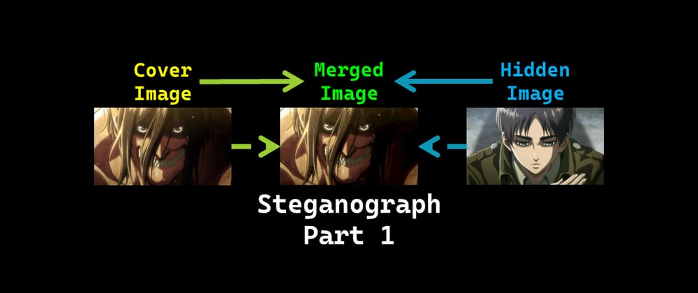
In simpler terms, steganography is akin to embedding a covert message within another overt message—in our case, hiding one image within another.
A digital image is an image composed of picture elements, also known as pixels, each with finite, discrete quantities of numeric representation for its intensity or gray level that is an output from its two-dimensional functions fed as input by its spatial coordinates denoted with x, y on the x-axis and y-axis, respectively - Wikipedia.
Imagine a digital image as an intricate mosaic composed of minuscule tiles, known as pixels. Each pixel contributes to the overall image by adding its own splash of color. The more pixels you have, the more vivid and detailed your image becomes.
Color models are tools central to color theory that define the color spectrum based on presence or absence of a few primary colors - onlinelibrary.wiley.com
Think of color models as the recipe books for digital artists. Just like mixing primary colors in art class, color models help us understand how to blend different amounts of red, green, and blue light to produce various hues. In this discussion, we'll focus on the RGB (Red-Green-Blue) color model, which is the cornerstone for reproducing a wide array of colors in digital media.
The name of the model comes from the initials of the three additive primary colors, red, green, and blue. The main purpose of the RGB color model is for the sensing, representation, and display of images in electronic systems, such as televisions and computers - Wikipedia.
Binary code is a system of representing information using only two symbols, typically 0 and 1 - Britannica
In the realm of digital images, each pixel's color information is represented by 8-bit binary digits. This means each pixel can display one of (2^8) or 256 possible colors.

In computing, the most significant bit (MSb) represents the highest-order place of a binary integer. Similarly, the least significant bit (LSb) is the bit position in a binary integer representing the binary 1s place of the integer - Wikipedia
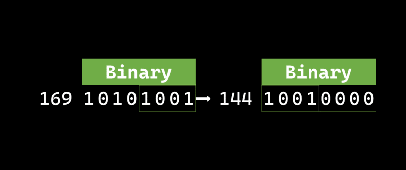
The concept of most significant bit (MSb) and least significant bit (LSb) is crucial here. Altering the MSb can have a profound impact on a pixel's color, while changes to the LSb are usually subtle.
The leftmost bit is the most significant bit. We change this bit and it will affect tremendously on the value. For example, we flip the leftmost bit of the binary value of 165 from 1 to 0 (from 10100101 into 00100101) it will change the decimal value from 165 into 37.
On the other hand, the rightmost bit is the least significant bit. We change this bit and it won't affect tremendously on the value. For example, we flip the rightmost bit of the binary value of 165 from 1 to 0 (from 10100101 into 10100100) it will change the decimal value from 165 into 164.

So, let's tie it all together: each pixel in a digital image comprises three color values (RGB), each represented by an 8-bit binary digit. We'll exploit the "insignificance" of the least significant bits to embed one image into another without causing noticeable changes to the host image. This is the magic key to image-based steganography. We'll change the less significant bits of one image to include the most significant bits of another.
In this technical dev blog post, you'll find:
So, buckle up for an exciting journey through the world of steganography!
Before diving into the technicalities of steganography, it's essential to set up your workspace properly. This ensures that you can effortlessly follow along with the examples and get the most out of this exploration. Whether you're a seasoned coder or just dipping your toes into the Python ecosystem, I've got you covered.
I've created a Google Colab-compatible Jupyter Notebook to make this process seamless. The notebook is designed with a user-friendly UI/UX and hides the raw code, so you can focus on learning. And the best part? The code is pre-validated to run without hitches on the first try!
If you're new to Google Colab or Python in general, don't worry! Here's an introductory video on Google Colab for Beginners to help you get started.
For those who are more experienced and might prefer to run the project locally, here are the Python package requirements to set up your environment:
Python 3.7.12
matplotlib==3.2.2
matplotlib-inline==0.1.3
matplotlib-venn==0.11.6
numpy==1.21.5
Pillow==7.1.2
scikit-learn==1.0.2
Once you have your environment set up, you'll be ready to delve into the world of steganography with me!
Before diving into the nitty-gritty details, it's crucial to understand the four types of binary value mappings that we'll be using:
Left-Half Bits Mapping (LHB Map)

Think of this mapping as a way to extract the left-half bits values from the cover image within the merged image.
Right-Half Bits Mapping (RHB Map)
This mapping aims to extract the left-half bits values of the hidden image from the merged image.
Whole Bits Mapping (MB Map)

This mapping is utilized to construct the whole bits values of the merged image, using the left-half bits values from both the cover and hidden images.
Possible Right-Half Bits Mapping (RRHB Map)

In this case, we'll randomly pick possible half bits values as we don't store the information about the half bits beforehand. The aim here is to construct the right-half bits values of the unmerged left-half bits image for both the unmerged cover and hidden images.
Now that we've understood the mapping types, let's look at how these mappings play a crucial role in hiding—or encoding—one image within another.

Here's a summarized flow of the encoding process:
Let's shift our focus to how we can extract—or decode—the hidden image from the merged image.

Here's a quick rundown of the decoding process:
Finally, let's look at how we can reconstruct the original images from their half-bit versions.

Here's how the reconstruction process works:
I hope these explanations provide a clearer understanding of the steganography techniques involved in hiding, revealing, and reconstructing images.
In this exploration, we'll limit our focus to only two image formats: PNG and JPEG. This limitation helps keep our exploration straightforward.
Before diving into the code's functionality, it's essential to get a grasp of its structure. Below is a snippet that outlines the main components of the code.
.
├── get_bits_dict(start: int, end: int, recon: bool = False) -> Dict[int, int]
├── get_merged_bits_array() -> np.ndarray
├── dict_to_nparray(d: dict) -> np.ndarray
├── dict_to_2darray(d: dict) -> np.ndarray
└── Steganograph
    ├── Object Attributes
    │     ├── ispng: bool
    │     ├── original_cover_image: numpy array
    │     ├── original_hidden_image: numpy array
    │     ├── left_half_bits_hidden_image: numpy array, default None
    │     ├── merged_image: numpy array, default None
    │     ├── unmerged_left_half_bits_cover_image: numpy array, default None
    │     ├── unmerged_left_half_bits_hidden_image: numpy array, default None
    │     ├── reconstructed_cover_image: numpy array, default None
    │     └── reconstructed_hidden_image: numpy array, default None
    ├──── Methods
    │     ├── encode(pos: str = 'upper_left')
    │     ├── decode(pos: str = 'upper_left')
    │     ├── encode_decode(pos: str = 'upper_left')
    │     ├── reconstruct()
    │     ├── encode_decode_recon(pos: str = 'upper_left')
    │     ├── is_two_images_identical(opt: int = 0) -> bool
    │     ├── save_image(opt: int = 0)
    │     ├── plot_original()
    │     ├── plot_left_half_bits()
    │     ├── plot_merged_image()
    │     ├── plot_unmerged_left_half_bits()
    │     └── plot_recon()
    └──── Class Attributes
          ├── __lhb_lookup: lhb #Left half bits array lookup
          ├── __rhb_lookup: rhb #Right half bits array lookup
          ├── __mb_lookup: mb #Merged bits 2D array lookup
          ├── __rrhb_lookup: rrhb #Reconstruction right half bits dict lookup
          ├── __format: tuple ('jpeg', 'png')
          ├── __rgb: tuple ('RGB', 'Red', 'Green', 'Blue')
          └── __pos: tuple ('upper_left', 'upper_right', 'lower_left', 'lower_right')
The code incorporates several helper functions tailored for the art of steganography. Here's a brief rundown:
get_bits_dict: This function produces a dictionary that maps an integer (ranging from 0 to 255) to another integer. The mapping varies based on whether the process is for reconstruction. In the standard case, it extracts the left-half bits, whereas for reconstruction, it extracts the right-half bits.
dict_to_nparray: Converting the dictionary from get_bits_dict into a numpy array facilitates faster lookup operations.
get_merged_bits_array: This function constructs a 2D array where each cell at index [i][j] holds the merged left-half bits (cover image) of i and the left-half bits (hidden image) of j.
dict_to_2darray: This works similarly to dict_to_nparray, but it reshapes the array into a 2D structure, particularly useful for image reconstruction.
Respective function callings for later:
__init__ Method:
The __init__ method initializes an instance of the Steganograph class.
cover_image_filepath: File path for the cover image (supports only JPEG or PNG formats).hidden_image_filepath: File path for the hidden image (supports only JPEG or PNG formats).Determine Image Formats: The method first determines the format (JPEG or PNG) of both the cover image and the hidden image using the imghdr.what() function. The formats are stored in format_ci and format_hi variables.
Validation: It checks whether both images have valid formats. If the formats don't match any in the class' __format attribute, it raises a TypeError.
Check Format Uniformity: It checks if both images have the same format. If not, it raises a TypeError.
PNG Format Flag: Sets the ispng flag to True if the format is PNG; otherwise, sets it to False.
Read Images: Reads the images into original_cover_image and original_hidden_image using the plt.imread() function from Matplotlib.
Invoke read_and_adjust_images: Calls the method read_and_adjust_images() to perform additional adjustments on the images.
Set Initial States: Initializes the other attributes to None, as these would be populated by other methods later.
read_and_adjust_images Method:
This method adjusts the read images for further processing, especially for PNG images. By the end of these methods, the class instance is well-prepared with loaded and adjusted images, and is ready for encoding and decoding operations.
ispng is True):
encode Method:
The encode method is responsible for creating a simple steganograph—merging a hidden image into a cover image in a way that it can later be extracted.
pos: Specifies where the hidden image will be located in relation to the cover image. Default is 'upper_left'.Position Validation: It validates whether the given position pos is one of the four pre-defined positions (upper_left, upper_right, lower_left, lower_right). If not, it raises a ValueError.
Get Left Half Bits: It calls get_left_half_bits to extract the left half-bits of the hidden image and stores them in the left_half_bits_hidden_image attribute.
Merge Half Bits: It then calls merge_two_half_bits to merge the modified hidden image with the cover image.
get_left_half_bits Method:
img_arr: The image array that you want to extract the left half-bits from.Lookup: It looks up the left half-bits of the image array img_arr using a pre-defined lookup table __lhb_lookup.
Return: It returns the left half-bits.
merge_two_half_bits Method:
pos: The position where the hidden image will be located in relation to the cover image.Copy Original Cover Image: It first creates a copy of the original cover image and stores it in self.merged_image.
Get Slicing Range: It calls the get_slicing method to determine the slice where the hidden image will be placed.
Merge the Half Bits: It merges the cover image and the modified hidden image together to create the final merged image (steganograph). It does this by using a pre-defined 2D lookup table __mb_lookup for each channel (RGB).
Type Casting: Finally, it casts the merged_image into 'uint8' type.
get_slicing Method:
large_shape: A tuple representing the shape of the larger array, which is the cover image in this case.small_shape: A tuple representing the shape of the smaller array, which is the hidden image.pos: The position where the hidden image will be located in relation to the cover image. Valid options are 'upper_left', 'upper_right', 'lower_left', and 'lower_right'.Extract Shape Information: The method first extracts the shape information of both the larger and smaller arrays. This information includes the number of rows and columns in each array.
Calculate Slicing Range: Based on the pos value, the function calculates the range in the larger array where the smaller array will be placed. This is done using numpy slice notation (np.s_).
Error Handling: If an invalid pos value is provided, a ValueError is raised.
Return: The function returns the calculated slicing range, which can be used as a slice object for numpy arrays. This slice object will then be used to place the hidden image in the specified position within the cover image.
By the end of the encode method, you'll have a steganograph where the hidden image is merged into the cover image at the specified position.
decode Method:
The decode method aims to break down the steganograph created by the encode method to recover the original hidden and cover images.
pos: This parameter specifies where the hidden image was embedded within the cover image. The default is 'upper_left'.Validation: First, the method checks if self.merged_image is None. If it is, it raises a TypeError. It also validates that the position pos is one of the acceptable positions. If not, a ValueError is raised.
Unmerge: It calls the unmerge_two_half_bits method to separate the cover and hidden images from the merged image.
unmerge_two_half_bits Method:
pos: Specifies the original position where the hidden image was embedded within the cover image.Slice Definition: Calls the get_slicing method to determine the slice range based on the pos value, i.e., where exactly the hidden image is located in the merged image.
Extract Left Half Bits of Cover Image: Uses the get_left_half_bits method to extract the left half bits of the merged image and assigns them to self.unmerged_left_half_bits_cover_image.
Extract Right Half Bits of Hidden Image: Similarly, it calls the get_right_half_bits method to extract the right half bits of the merged image. However, it does so only for the area specified by the slicing range returned by get_slicing.
get_right_half_bits Method:
img_arr: The image array that you want to extract the right half-bits from.Lookup: It looks up the right half-bits of the image array img_arr using a pre-defined lookup table __rhb_lookup.
Return: It returns the right half-bits.
In summary, the decode method and its supporting methods work together to reverse the steganographic process, extracting the hidden image and cover image from the merged image.
reconstruct Method:
The reconstruct method aims to restore the original cover and hidden images from their left-half bits images, which were previously separated during the decoding process.
Validation: The method checks that self.unmerged_left_half_bits_cover_image and self.unmerged_left_half_bits_hidden_image are not None. If either of them is None, it raises a TypeError, prompting you to run the decode() method first.
Reconstruct Cover Image: The reconstruct_right_half_bits method is called to reconstruct the right-half bits of the cover image. The reconstructed image is stored in self.reconstructed_cover_image.
Reconstruct Hidden Image: Similarly, the reconstruct_right_half_bits method is used to reconstruct the right-half bits of the hidden image. The reconstructed image is stored in self.reconstructed_hidden_image.
reconstruct_right_half_bits Method:
im_arr: The left-half bits of an image as a numpy array.seed: A seed for the random number generator, defaulting to 1999.Random Seed: The np.random.seed function is used to set the random seed to ensure that the random process is reproducible.
Flattening Image: The ravel() method is used to flatten the im_arr, essentially turning it into a one-dimensional array (flat_im_arr).
Random Indices: A random set of indices (random_indices) is generated using np.random.randint, with the size of the array based on the shape of flat_im_arr. This will simulate the random selection of right-half bits for each corresponding left-half bit.
Reconstruction: The lookup table __rrhb_lookup is used in conjunction with random_indices to get a set of right-half bits for each corresponding left-half bit in flat_im_arr. The result (reconstructed_flat) is a one-dimensional array containing the reconstructed right-half bits.
Reshaping: The reconstructed one-dimensional array is reshaped back into its original shape (shape) to form the reconstructed image.
Type Casting: Finally, the numpy array is cast to the type 'uint8'.
Return: The reconstructed image, now having both left and right half-bits, is returned.
In summary, the reconstruct method and its sub-method reconstruct_right_half_bits work together to restore the original cover and hidden images from their left-half bits versions. This final step completes the round-trip process of encoding, decoding, and reconstructing the images.
For the complete code and a more detailed walkthrough, check out the Jupyter Notebook linked below:
Having delved into the theory and implementation details, it's time to see our steganography technique in action. We'll examine the visual changes and quality metrics at each stage of the process—encoding, decoding, and reconstruction.
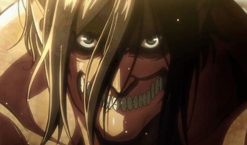
First, let's consider our "Cover Image" and "Hidden Image." The image below serves as our cover:

Next, we have the hidden image:

For a deeper understanding, let's examine the RGB plot of these images. Click on the image below to enlarge it.

After encoding, we obtain two new images: the "Left Half Bits Hidden Image" and the "Merged Image."
The encoded "Left Half Bits Hidden Image" noticeably loses some quality compared to the original hidden image. For instance, the gradients do not blend as smoothly.

Here's the RGB plot for a more in-depth analysis:

At first glance, the "Merged Image" looks almost identical to the original cover image. However, a keen eye might spot a subtle face formation in the upper-left corner.
For a more analytical view, let's check the RGB plot:

Next, we decode the merged image to obtain the "Unmerged Left Half Bits Cover Image" and the "Unmerged Left Half Bits Hidden Image." Both of these images show a loss in quality and coherence, similar to what we observed with the left half bits hidden image.


Take a look at the RGB breakdown for further insights:

Finally, we move on to the reconstruction stage, where we aim to approximate the original images as closely as possible.
When compared to the unmerged version, the reconstructed cover image appears slightly brighter. However, it's essential to note that the image quality is still not on par with the original. Gradients, for example, do not blend as smoothly as they should.

A similar trend is observed in the reconstructed hidden image. Though somewhat brighter than the unmerged version, the quality still falls short of the original.

For a more analytical perspective, let's examine the RGB plots of these reconstructed images:

For the evaluation, I utilized the Root Mean Square Error (RMSE) and Mean Absolute Error (MAE) metrics. These metrics help to quantify the differences between the images at different stages of the steganography process. While I can't speak to their application in formal steganalysis, they do offer a way to gauge the effectiveness of the encoding and decoding steps. If you have insights or recommendations on other metrics that might be more suitable, especially from a steganalysis point of view, feel free to share.
For instance, comparing the "Left Half Bits Hidden Image" with the original hidden image yielded the following results:
RMSE    : 8.868079206151936
MAE     : 7.579809053497942
This indicates that the two images are indeed different. However, when comparing the "Left Half Bits Hidden Image" with the "Unmerged Left Half Bits Hidden Image," the result was:
RMSE    : 0.0
MAE     : 0.0
This confirms that the encoding and decoding processes were executed correctly, as the two images are logically the same.
Once again, for the complete code and walkthrough, just run the Jupyter Notebook linked below:
This concludes the "Results and Visualization" section, where we've explored the visual aspects and quality metrics of images at every stage—encoding, decoding, and reconstruction. These visual examples and metrics serve as a comprehensive evaluation of our steganography technique.
In this section, we delve into the limitations of the current implementation and discuss opportunities for future enhancements.
Image Channel Handling: The code is designed to work specifically with RGB color spaces. This makes it less versatile when dealing with other color spaces or grayscale images.
Limited File Format Support: The code currently supports only PNG and JPEG formats, potentially excluding users with images in other formats.
Code Complexity: The codebase is somewhat intricate, which might make it less accessible for individuals who are not familiar with the project's specifics.
Error Handling: While some error-handling mechanisms exist, they may not be comprehensive enough to address all potential edge cases.
Hard-Coded Values: The presence of hard-coded values in the code reduces its flexibility and adaptability.
Google Colab Dependency: The code relies on Google Colab-specific libraries, making it less portable for users who may prefer other development environments.
Lack of Modularization: The code is not modular, which could complicate future efforts to extend its functionality or maintain it.
Enlightening and Challenging: Our exploration into steganography has been a revealing journey, showcasing both the potential and the challenges of this field.
Practical Applications: We demonstrated how one image could be hidden within another, a technique with various real-world applications such as digital watermarking and secure communications.
Identified Limitations: Like any scientific endeavor, our work has its constraints, from the limitations in color channel handling to dependencies on specific platforms like Google Colab. These offer avenues for future research and refinement.
Bit Manipulation: One of the technical milestones of this project is the successful implementation of bit manipulation techniques to encode and decode images.
Visual Proof: We provided visual examples to demonstrate our techniques in action. While the hidden image is not perfectly concealed in our experiments, we believe that in scenarios with more detailed and crowded cover images, the concealment could be more effective.
Quantitative Analysis: We've used metrics such as RMSE and MAE to measure differences between original and manipulated images. While these metrics offer insights, they may not be specifically tailored for steganalysis. If you have expertise in steganalysis, your feedback in the comments would be highly valuable.
What seemed like a straightforward task—hiding one image within another—unfolded into a labyrinth of complexities. The project has underscored the intricacies of image manipulation and bit-level operations.
The limitations we've faced have highlighted the importance of robust and flexible code. As we continue to refine this project, the lessons learned here will be invaluable.
The world of steganography is vast, and there's so much more to explore. Your feedback and contributions are not just welcome but are essential for the continuous improvement of this project.
The avenues for future work are promising. They range from refining the current code to make it more versatile to exploring more advanced steganographic techniques. With ongoing research and collaboration, the sky is the limit for what can be achieved.
Exploring Steganography In The Wild


